Geoanalysis with Power BI: Transform Latitude and Longitude into Country, State, and Territory

3 November 2024 - Written by Markus Böhm

Geographic data

Business data frequently includes geographic information, such as country, state, city, and zipcode of customers. This data enables visualization of sales performance by country in detailed tables or dynamic maps.

Sometimes geographic data consists solely of a geographic point represented by two numbers: latitude and longitude. Now this is a geographic point:

49.580614486244784 11.029701285355571

How do you know where this point is on earth? To which country does it belong? To which city?

Classify Geographic Points

If you are familiar with geographic coordinates, then you identify the latitude as a location 49° north of the equator and the longitude as 11° east of London. By entering these coordinates into Google Maps, you can find that this geographic point is actually located in the country Germany, the state Bavaria and the city Erlangen. This process can be used to manually enrich the classification of geographic points.

But what if there are a lot of geographic points, such as the locations of bike rentals, photos taken or goods stored? You can utilize GIS software or libraries in languages like Python, R, or JavaScript. But can Power BI perform this task?

What Do You Need to Use Power BI for Geographical Analysis?

To get started, you need a definition of the territory, typically represented by a list of geographic points along its border. You can create this list yourself using Google Maps, or you can utilize an existing list in a GeoJSON or CSV format.

Next, you will need code to determine whether your points fall within the defined border of the territory.

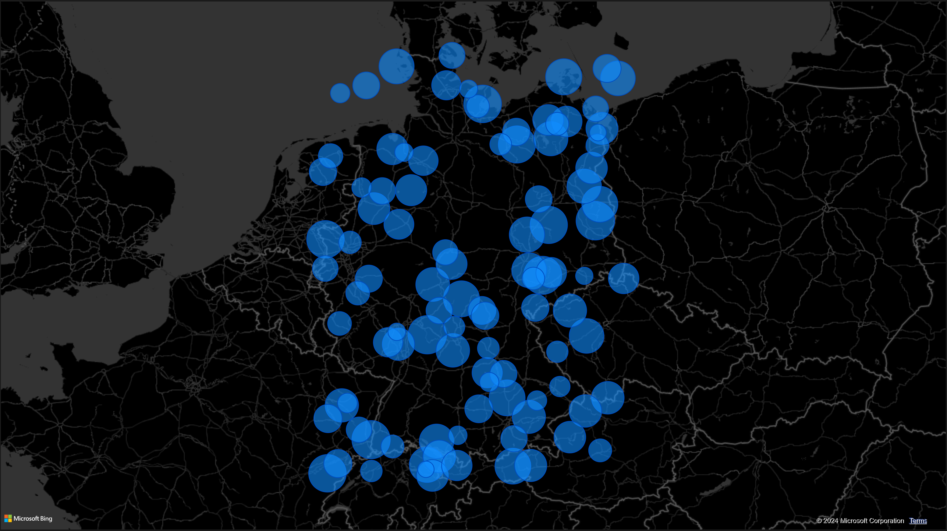
You can implement this logic directly in Power BI. This approach allows you to make sense of numerous geographic points and visualize them effectively like this.

Geometry Background

The task we will solve is common in geometry and geography. It is called Point in Polygon. French mathematician Camille Jordan proved that a closed curve separates an interior from an exterior. By crossing the curve one will always go from inside to outside or vice versa.

The idea of the algorithm is as follows:

• start far away to ensure you are outside
• from there approach the point
• count how often you cross the closed curve on your way
• if this number is odd when you reach the point, the point is inside

To keep it simple:

• The closed curve is a polygon
• The way to the point is straight and horizontal

Here is a territory and some points. The territory is grey and shaped like the letter M. Red points are on the border of the territory. They define the border and the territory. A black line connects the red points and forms the border of the territory.

One wants to know whether the blue, brown, green and purple points lie inside or outside of the territory.

Let’s add the horizontal rays and count the number of intersections.

For brown and blue we find 1 and 3 intersections, respectively. 1 and 3 are odd numbers, that is brown and blue are inside. For purple and green we find 2 and 4 intersections. 2 and 4 are even numbers, meaning purple and green are outside. That was easy!

Now we want to teach Power BI how to compute this.

Intersection with a Line

Intersections of lines is basic geometry: Line-line intersection.

Let’s focus on the blue point and start with a full horizontal line through the blue point. Which edges might the straight blue line cross?

The blue line can only cross edges which are on the same horizonal level as the blue point. It can only cross edges whose end points are one above and one below the blue point. The blue horizontal line crosses 4 edges. They are shown in black. The edges which are not intersected are shown in grey.

If we name the point P = (x_P, y_P) and the edges of the line segment A = (x_A, y_A) and B = (x_B, y_B) then this is the formula for it:

y_A < y_P ≤ y_B   or   y_B < y_P ≤ y_A

Intersection with a Ray

We want to count the intersections to the right of the point only. That are the intersections with a ray or half line from the point to the right.

But which of the edges are crossed to the right of the point P?

Let’s focus on one edge. The end of the edge are named A and B. Our point to test is P. And the intersection of the horizontal blue line with the edge is C. Each of the points has coordinates A = (x_A, y_A), B = (x_B, y_B), C = (x_C, y_C) and P = (x_P, y_P).

The intersection C is to the right of the point P if the x coordinate of the intersection C is greater than the x coordinate of the point P.

x_P < x_C

With a bit of calculus one can compute x_C. The condition becomes:

x_P < x_A + (x_B − x_A) ∙ (y_P − y_A) ∕ (y_B − y_A)

Resulting Formula

With the help of geometry we found that for one point P and a polygon we have to check for every edge of the polygon these two conditions

y_A < y_P ≤ y_B   or   y_B < y_P ≤ y_A

x_P < x_A + (x_B − x_A) ∙ (y_P − y_A) ∕ (y_B − y_A)

If both are true then there is a crossing of the horizontal line with the edge to the right of the point P.

We count the number of crossed edges. If this number is odd the point P lies within the polygon, if the number is even the point P lies outside the polygon.

Prepare the Territory for Power BI

The fastest way to a territory is to create it yourself. In Google Maps I clicked some points around the border of Germany. A right click displays the coordinates. Copy these into a text editor and save in CSV-format.

54.79966235421943, 9.57374171147848
50.774397057471255, 6.166678735781409
49.017641449798994, 8.770679188531576
47.61366890494342, 7.6509649976271
47.61719462756167, 13.154404836703625
48.568982471110836, 13.432844355930914
50.313066683987174, 11.947256819488164
51.14647283023247, 14.9061062126246
54.31174216822144, 13.18257644864103
54.79966235421943, 9.57374171147848

Power BI can load this. Power Query can join the adjacent points to form border lines. The result of the data preparation looks like this.

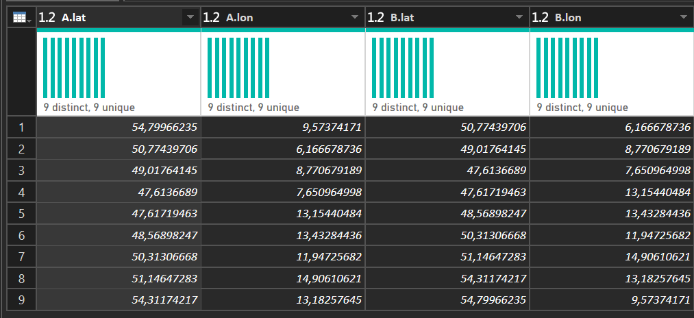
Each row contains the starting point A and the ending point B of one edge. The ending point of one edge is the starting point of the next edge. In total we have 9 edges forming a polygon.

Create some Points

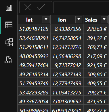
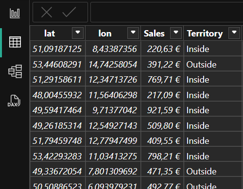
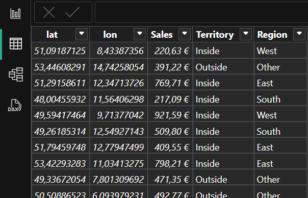
We want to enrich geographic points by assigning territories to them. We could use real data. For this post I generated some random points in Power Query and loaded them into the table Points. They have three values: Latitude, Longitude and Sales. Latitude and longitude are needed to know where the point is. Sales is an example of additional data we may have for the point.

On a map these points look like this. Each bubble is located at its latitude and longitude. The size of the bubble grows with the attribute sales.

One Territory in Power BI

Now we enhance the table Points. We use the prepared polygon data in the table Territory to classify each point.

We do this by defining a calculated column Points[Territory] in the table Points.

The DAX code first stores the latitude and the longitude in the variables x and y.

Then it filters the table Territory by applying our two conditions. It keeps only the edges which are crossed by a ray casted to the right. These edges are counted. If the resulting number is odd the point is inside. Otherwise it is outside.

Territory = 
VAR y = Points[lat] 
VAR x = Points[lon]
VAR Inside = 
    ISODD(COUNTROWS(
        CALCULATETABLE(Territory,
            VAR xA = Territory[A.lon]
            VAR yA = Territory[A.lat]
            VAR xB = Territory[B.lon]
            VAR yB = Territory[B.lat]
            RETURN 
                ((yA < y && y <= yB) || (yB < y && y <= yA))  
                && 
                (x < (xB-xA)*(y-yA)/(yB-yA) + xA)
        )
    ))
RETURN IF(Inside,"Inside","Outside")

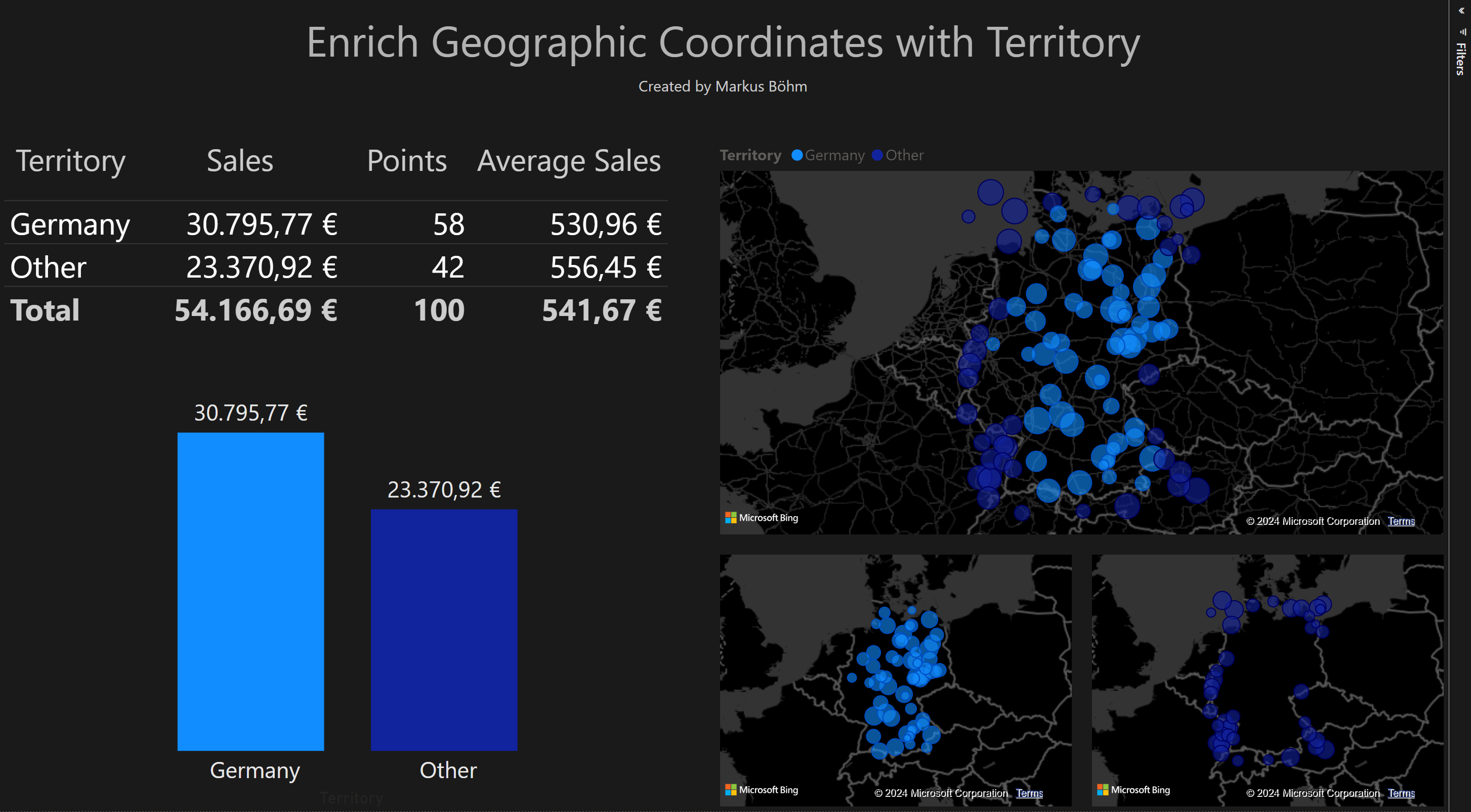
Now each geographical point is enriched by a territory.

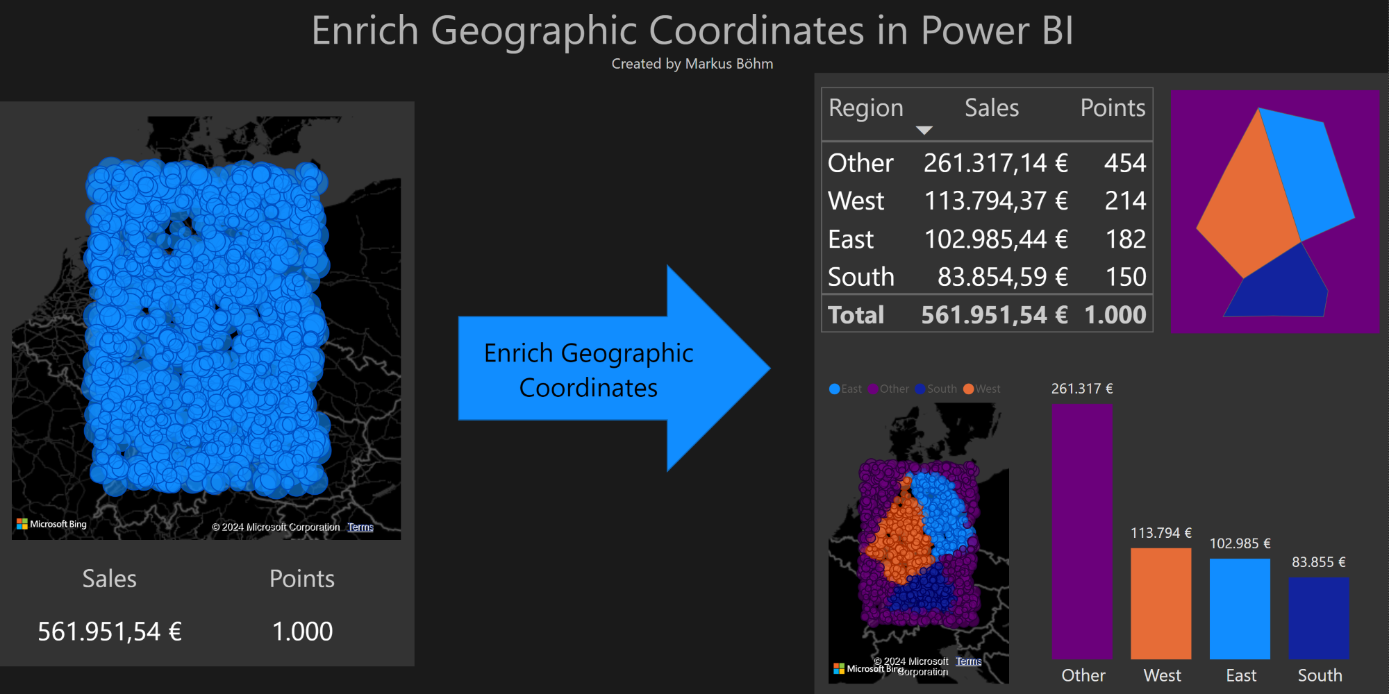
This new column can be used to analyse the data. We color the inside points in light blue and the outside points in dark blue.

Not only gives the data in a map more insights. We can use our new column in a table chart or a column chart, too.

We can count the number of points inside. We can sum the sales of the inside points.

Prepare Multiple Territories for Power BI

Up to now we had one territory. Our business question was:

Is the point inside or outside of this territory?

What if we have more than one territory? Then our question may become:

Inside which territories is our point?

Let’s try this!

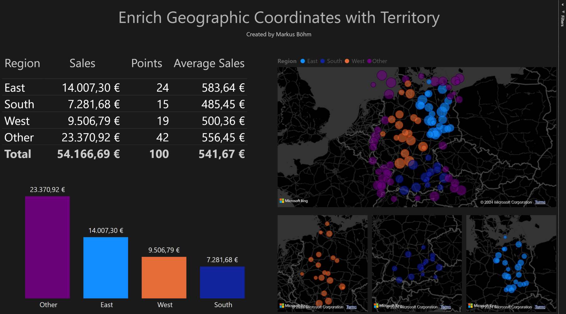
We use the previous territory but split it in three parts. We name the territories West, South, and East.

54.79966235421943, 9.57374171147848, West
50.774397057471255, 6.166678735781409, West
49.017641449798994, 8.770679188531576, West
50.313066683987174, 11.947256819488164, West
54.79966235421943, 9.57374171147848, West
49.017641449798994, 8.770679188531576, South
47.61366890494342, 7.6509649976271, South
47.61719462756167, 13.154404836703625, South
48.568982471110836, 13.432844355930914, South
50.313066683987174, 11.947256819488164, South
49.017641449798994, 8.770679188531576, South
50.313066683987174, 11.947256819488164, East
51.14647283023247, 14.9061062126246, East
54.31174216822144, 13.18257644864103, East
54.79966235421943, 9.57374171147848, East
50.313066683987174, 11.947256819488164, East

As before we load this into Power BI and join the adjacent points to form the edges of the border. The resulting table Region looks like this.

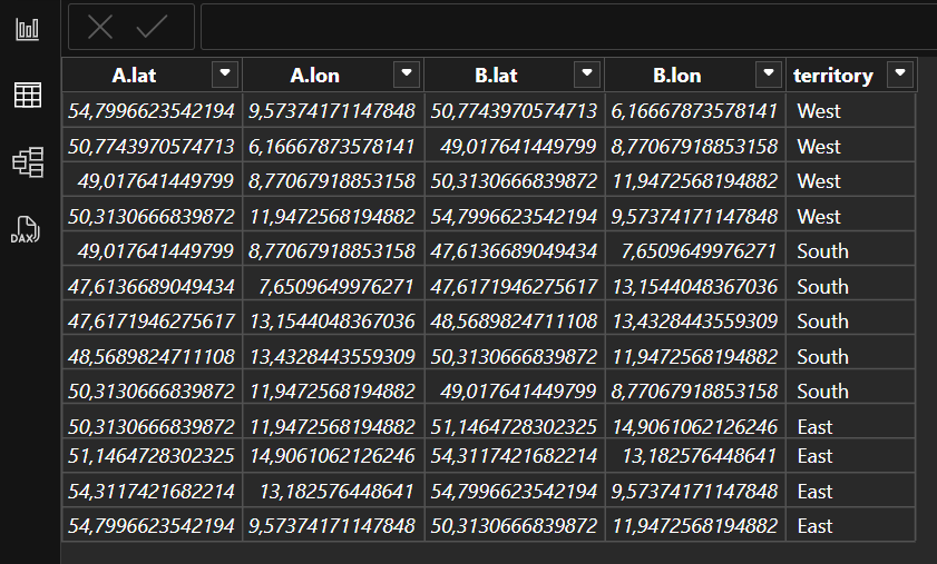
Each row contains a starting point A and an ending point B of one edge. The ending point of one edge is the starting point of the next edge. Each edge belongs to one of the territories West, South, and East. The territories have four or five edges each. These edges form a polygon per territory.

Multiple Polygons in Power BI

Now we enhance the table Points once more. We use the prepared multi-polygon data in the table Region to classify each point.

We do this by defining a calculated column Points[Region].

The DAX code is very similar to the code for one polygon. But now it uses one more iteration. We iterate over the three possible values West, South, and East of the Region[region]. This is done by the FILTER(VALUES(Region[region]),…). So we perform the code from above for each of our three polygons.

Our regions are disjunct, i.e. each point can be inside of one region only. If it is outside of all regions we return the value Other.

Region = 
VAR y = Points[lat] 
VAR x = Points[lon]
VAR Inside = 
    FILTER(
        VALUES(Region[region]),
        ISODD(COUNTROWS(
            CALCULATETABLE(Region,
                VAR xA = Region[A.lon]
                VAR yA = Region[A.lat]
                VAR xB = Region[B.lon]
                VAR yB = Region[B.lat]
                RETURN 
                    ((yA < y && y <= yB) || (yB < y && y <= yA))  
                    && 
                    (x < (xB-xA)*(y-yA)/(yB-yA) + xA)
            )
        ))
    )
RETURN COALESCE(Inside,"Other")

Now each geographical point is enriched by a one of the three regions.

This new column can be used to analyse the data in more detail. We use different colors for the points in the three regions and for the outside points.

We used the same table and the same column chart as above but now with 3 regions instead of one.

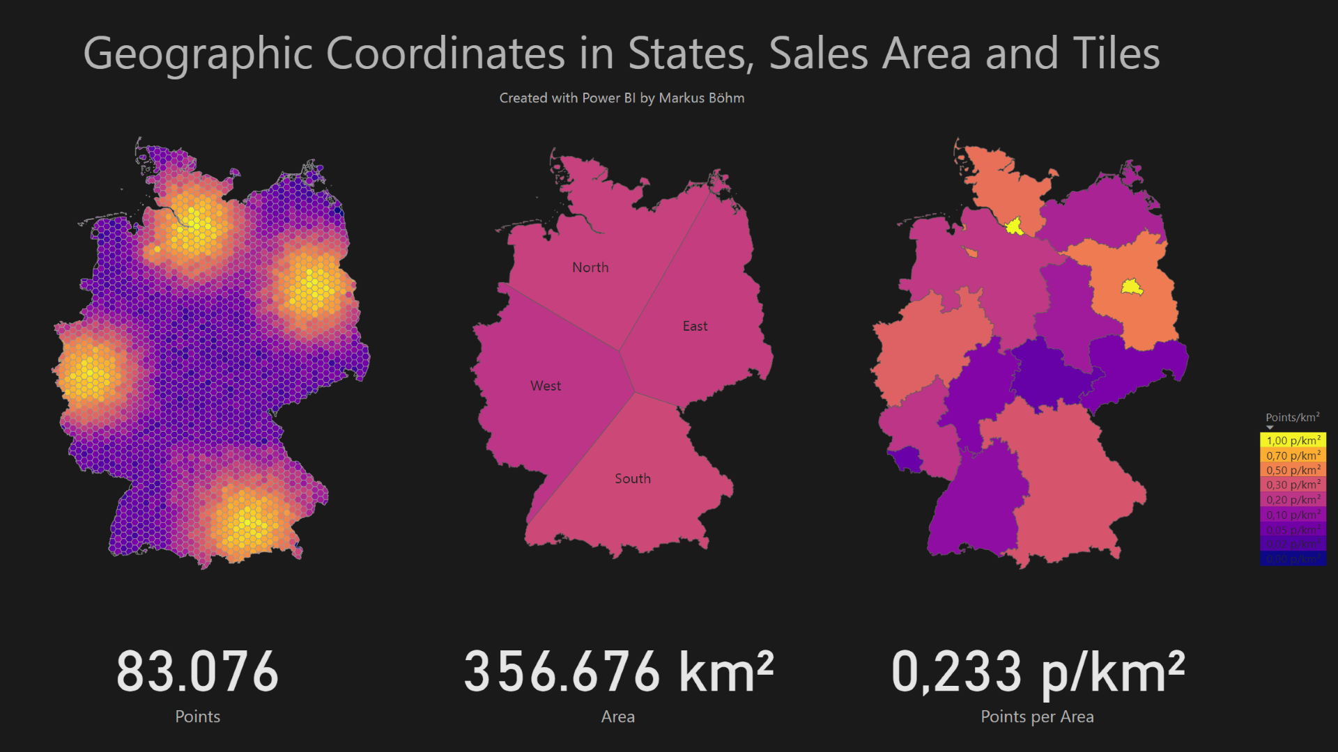
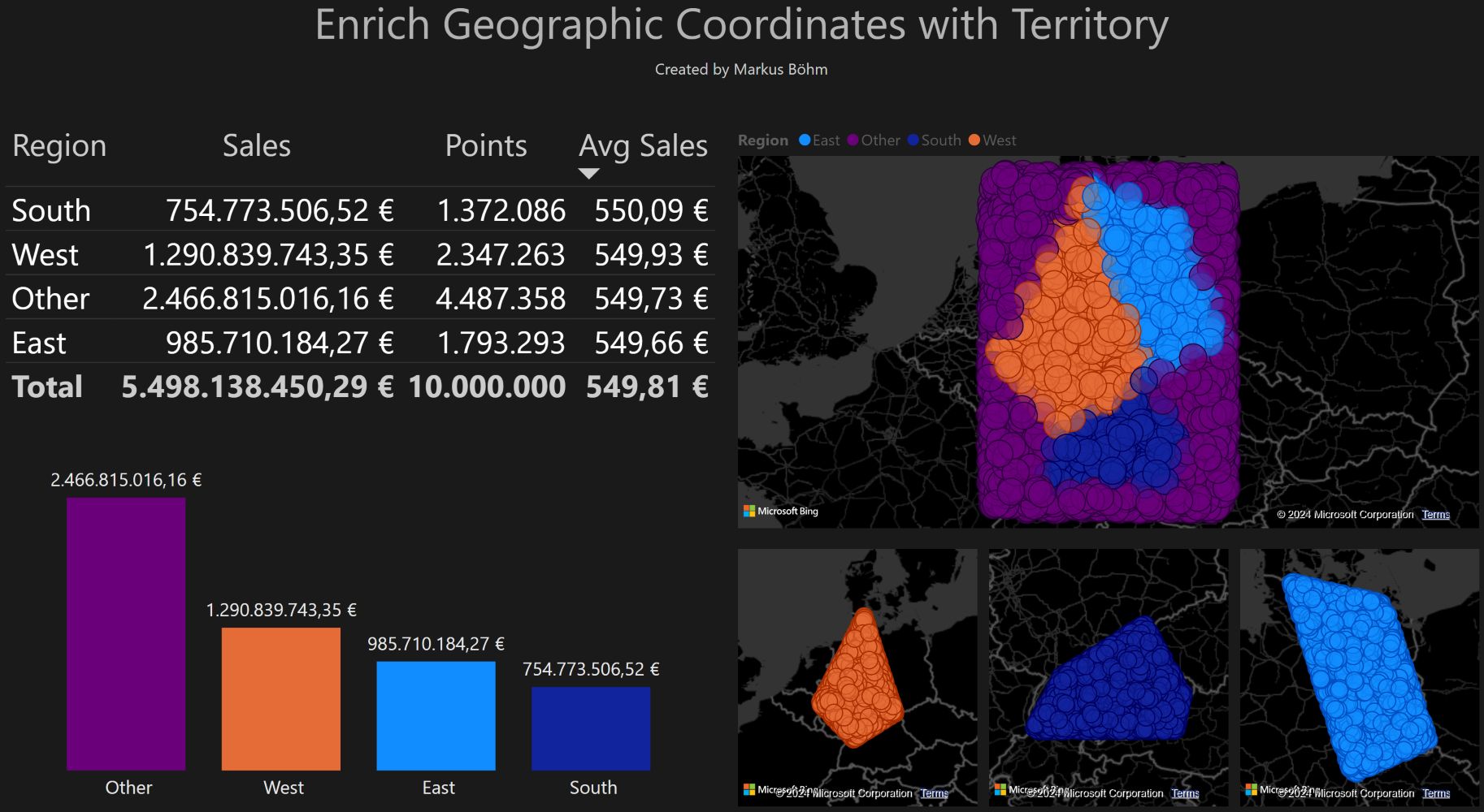
Performance

This algorithm works well with millions of points. Here is the same analysis but with 10 million points instead of 100.

Conclusions

One can enrich geographic coordinates with semantic data by using polygons for territories. This is a common approach in different languages. Currently there is no standard function in Power Query or DAX to do this. This post explained how it can be done in Power BI. With some lines of DAX code one can do this fast and reliable.

I hope you remember this if you come across geographic data next time!

If you like this post

I would like to hear from you if you have a use case for Geoanalysis in Power BI.

You can help spread this idea by sharing this post or this LinkedIn post or this X post.

If there is interest I may prepare another post with more details.

You have data with geographic points and you can share it with me and the public? I would like to do a post with some real data!